Data Analysis🔎

Load the Packages

library(tidyverse)

── Attaching core tidyverse packages ──────────────────────── tidyverse 2.0.0 ──
✔ dplyr     1.1.4     ✔ readr     2.1.5
✔ forcats   1.0.0     ✔ stringr   1.5.1
✔ ggplot2   3.5.1     ✔ tibble    3.2.1
✔ lubridate 1.9.4     ✔ tidyr     1.3.1
✔ purrr     1.0.2     
── Conflicts ────────────────────────────────────────── tidyverse_conflicts() ──
✖ dplyr::filter() masks stats::filter()
✖ dplyr::lag()    masks stats::lag()
ℹ Use the conflicted package (<http://conflicted.r-lib.org/>) to force all conflicts to become errors

library(plotly)

Attaching package: 'plotly'

The following object is masked from 'package:ggplot2':

    last_plot

The following object is masked from 'package:stats':

    filter

The following object is masked from 'package:graphics':

    layout

library(ggplot2)
library(rnaturalearth)
library(htmlwidgets)

Load the Cleaned Data

load("data/olympics_dfclean.Rdata")

Inspect the Cleaned Data

glimpse(olympics_dfclean)

Rows: 252,565
Columns: 7
$ athlete_name <chr> "A Dijiang", "A Lamusi", "Gunnar Aaby", "Edgar Aabye", "C…
$ year         <int> 1992, 2012, 1920, 1900, 1932, 1932, 1952, 2000, 1996, 200…
$ sex          <fct> M, M, M, M, F, F, M, M, F, F, M, M, M, M, M, M, M, M, M, …
$ country      <fct> "China", "China", "Denmark", "Denmark/Sweden", "Netherlan…
$ sport        <fct> "Basketball", "Judo", "Football", "Tug-Of-War", "Athletic…
$ medal        <fct> No medal, No medal, No medal, Gold, No medal, No medal, N…
$ event        <chr> "Basketball Men's Basketball", "Judo Men's Extra-Lightwei…

Question1-Analysis

How has gender equality in athlete participation evolved across Olympic history, and what trends are visible in the representation of men and women from 1896 to 2024?

Yr_num <- olympics_dfclean |>
  distinct(athlete_name, year, sex) |>  # Ensure each athlete is only counted once per year per sex (avoid duplicates)
  group_by(year, sex) |>
  summarise(athlete_count = n()) |>  # Count the number of athletes per year and gender
  group_by(year) |>  # Group again by year to compute total athletes in each Olympic year
  mutate(total = sum(athlete_count),  #  Total athletes for that year
    percentage = round((athlete_count / total) * 100, 1)) |>  # Percentage of each gender
    arrange(year, sex)  

`summarise()` has grouped output by 'year'. You can override using the
`.groups` argument.

# View the table
Yr_num

# A tibble: 61 × 5
# Groups:   year [31]
    year sex   athlete_count total percentage
   <int> <fct>         <int> <int>      <dbl>
 1  1896 M               176   176      100  
 2  1900 F                23  1215        1.9
 3  1900 M              1192  1215       98.1
 4  1904 F                 6   642        0.9
 5  1904 M               636   642       99.1
 6  1906 F                 6   838        0.7
 7  1906 M               832   838       99.3
 8  1908 F                44  2008        2.2
 9  1908 M              1964  2008       97.8
10  1912 F                53  2386        2.2
# ℹ 51 more rows

Key Insight:

The Olympic Games have transformed in terms of gender representation from 1896 to 2024. Initially, female participation was minimal, with women making up less than 3% of athletes before 1920. This changed gradually, reaching about 10–15% by the 1960s. Significant growth occurred in the 1970s, followed by more increases in the 1980s and 1990s. By 2000, women represented 38.2% of athletes, climbing to 44.3% by 2012. The most recent Paris Olympics also saw a female athlete representation of 47.8% in 2020 and 49.1% in the 2024 Paris Olympics.

Question1-Visualization

p1 <- ggplot(Yr_num, aes(
  x = factor(year),
  y = athlete_count,
  fill = sex,
  text = paste0("Year: ", year,
                "<br>Sex: ", ifelse(sex == "F", "Female", "Male"),
                "<br>Athletes: ", athlete_count))) +
  geom_col(position = "stack", color = "white") +  
  scale_fill_manual(
    values = c("F" = "#FFB6C1", "M" = "#87CEFA"),  
    labels = c("F" = "Female", "M" = "Male"),
    name = "Sex") +
  labs(title = "Olympic Participation by Gender (1896–2024)",
    subtitle = "Light and shiny color palette for gender-based participation",
    x = "Olympic Year",
    y = "Number of Athletes",
    caption = "Source: Kaggle | Author: Brandon") +
  theme_light(base_size = 12) +
  theme(plot.title = element_text(face = "bold", size = 14),
    plot.subtitle = element_text(size = 11, color = "gray30"),
    legend.title = element_text(face = "bold"),
    plot.caption = element_text(size = 10, hjust = 0),
    axis.text.x = element_text(angle = 45, hjust = 1))


p1_plotly <- ggplotly(p1, tooltip = "text")

p1_plotly

# Save the interactive plot
htmlwidgets::saveWidget(p1_plotly, "out/interactive_plot1.html", selfcontained = TRUE)

Question2-Analysis

Among the most popular Olympic sports since 1992, which show a balanced gender representation, and which show persistent gender disparities?

# Get top 10 sports by total number of athletes
top_sport <- olympics_dfclean |>
  filter(year >= 1992) |> # Focus only on Olympic years from 1992 onward
  distinct(athlete_name, year, sport, sex) |> # Remove duplicate entries 
  group_by(sport) |>
  summarise(athlete_num = n()) |> # Count number of unique athlete entries per sport
  top_n(10, athlete_num) # Select top 10 sports with the highest participation

# Get the gender breakdown within those top sports
gender_sport <- olympics_dfclean |>
  filter(year >= 1992, sport %in% top_sport$sport) |>  
  distinct(athlete_name, year, sport, sex) |>
  group_by(sport, sex) |>
  summarise(athlete_num = n()) |>
  group_by(sport) |>  # Group again to calculate percentage per sport
  mutate(total = sum(athlete_num), #Create a new column 'total': total number of athletes (male + female) in each sport
    percentage = round((athlete_num / total) * 100, 1)) |> # Create a new column 'percentage': % of athletes by gender in that sport
  arrange(sport, sex)

`summarise()` has grouped output by 'sport'. You can override using the
`.groups` argument.

gender_sport

# A tibble: 20 × 5
# Groups:   sport [10]
   sport     sex   athlete_num total percentage
   <fct>     <fct>       <int> <int>      <dbl>
 1 Athletics F            8160 18372       44.4
 2 Athletics M           10212 18372       55.6
 3 Cycling   F             956  3376       28.3
 4 Cycling   M            2420  3376       71.7
 5 Football  F            1516  4042       37.5
 6 Football  M            2526  4042       62.5
 7 Handball  F            1429  3037       47.1
 8 Handball  M            1608  3037       52.9
 9 Hockey    F            1563  3341       46.8
10 Hockey    M            1778  3341       53.2
11 Judo      F            1471  3531       41.7
12 Judo      M            2060  3531       58.3
13 Rowing    F            1875  5004       37.5
14 Rowing    M            3129  5004       62.5
15 Sailing   F            1202  3538       34  
16 Sailing   M            2336  3538       66  
17 Shooting  F            1328  3489       38.1
18 Shooting  M            2161  3489       61.9
19 Swimming  F            3515  7900       44.5
20 Swimming  M            4385  7900       55.5

Key Insight:

The above analysis indicates that gender representation in the top 10 Olympic sports since 1992 has become more balanced in some areas, although notable differences still exist. Sports such as Handball and Hockey display relatively even participation between men and women, with women representing approximately 47% of all athletes. On the contrary, some sports, like Cycling and sailing, have a lower female representation. For instance, in Cycling, women account for around 28.3% of participants, with a difference of over 1,464 athletes compared to men. Female participation rates in widely participated sports like Athletics and Swimming are around 44–45%, which indicates that gradual movement toward greater inclusion.

Question2-Visualization

p2 <- ggplot(gender_sport, aes(x = reorder(sport, -total), y = athlete_num, fill = sex)) +
  geom_bar(stat = "identity", position = "stack", width = 0.7) +
  scale_fill_manual(values = c("F" = "#f7b6d2", "M" = "#aec7e8"), labels = c("Female", "Male")) +
  labs(title = "Gender Distribution in Top 10 Olympic Sports (Since 1992)", 
       x = "Sport", y = "No. of Athletes", caption = "Source: Kaggle | Author: Brandon") +
  theme_light(base_size = 13) +
  theme(plot.title = element_text(face = "bold", size = 13, hjust = 0.5),
        axis.text.x = element_text(angle = 45, hjust = 1),
        legend.position = "top",
        legend.title = element_text(size = 12),
        legend.text = element_text(size = 12))

ggplotly(p2)

p2_plotly <- ggplotly(p2)

# Save the interactive plot
htmlwidgets::saveWidget(p2_plotly, "out/interactive_plot2.html", selfcontained = TRUE)

Question3-Analysis

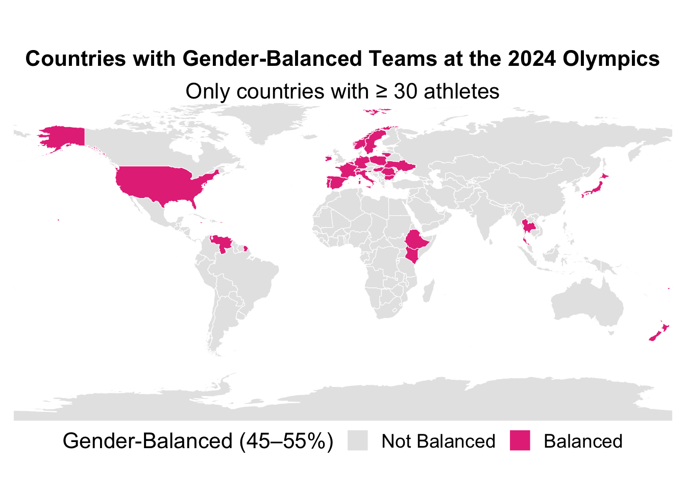
Which countries had gender-balanced athlete representation (45%–55% female) at the 2024 Olympics, and how are these countries distributed globally?

female_participation <- olympics_dfclean |>
  filter(year == 2024) |>  
  distinct(country, sex, athlete_name) |>  # Ensure each athlete is counted only once per country/sex
  group_by(country, sex) |>
  summarise(athletes_num = n()) |>  # Count athletes by country and gender
  pivot_wider( names_from = sex,
    values_from = athletes_num,
    values_fill = 0) |>  # Reshape so that the Female and Male athlete are separate columns
  mutate(total = F + M,  # Create a total column for calculating total athletes per country
    percentage_female = round(F / total * 100, 1))  # Calculate % of female athletes

`summarise()` has grouped output by 'country'. You can override using the
`.groups` argument.

#Keep countries with at least 30 total athletes
female_participation_filtered <- female_participation |>
  filter(total >= 30)

#Identify gender-balanced countries (45–55% female)
balanced_countries <- female_participation_filtered |>
  filter(percentage_female >= 45 & percentage_female <= 55) |>  # Filter to near-balance
  mutate(diff_from_50 = abs(percentage_female - 50)) |>  # How close each country is to 50%
  arrange(diff_from_50)  # Sort from most balanced to least (within the range above)

balanced_countries

# A tibble: 31 × 6
# Groups:   country [31]
   country         F     M total percentage_female diff_from_50
   <fct>       <int> <int> <int>             <dbl>        <dbl>
 1 Slovenia       47    47    94              50          0    
 2 Belgium        88    89   177              49.7        0.300
 3 Spain         202   198   400              50.5        0.5  
 4 Portugal       37    38    75              49.3        0.700
 5 Germany       225   232   457              49.2        0.800
 6 Jamaica        32    33    65              49.2        0.800
 7 France        295   306   601              49.1        0.900
 8 Romania        47    49    96              49          1    
 9 Ukraine        69    72   141              48.9        1.10 
10 New Zealand   101   107   208              48.6        1.40 
# ℹ 21 more rows

# Count how many countries had at least 30 athletes 
n_total_countries <- n_distinct(female_participation_filtered$country)
n_total_countries

[1] 66

# Count how many countries are gender-balanced
n_balanced <- nrow(balanced_countries)
n_balanced

[1] 31

Key Insight:

The above analysis looked at 2024 Olympic teams and identified countries with gender-balanced participation (45%–55% female athletes). among countries with at least 30 total athletes, 31 countries fell within this range. At the top of the list, Slovenia had a perfect 50/50 split between men and women (47 each). Countries like Belgium, Spain, Portugal, and Germany also had close-to-even splits, ranging from 49.2% to 50.5% female. Even larger delegations such as France, the United States, and Great Britain achieved balanced representation.

Question3-Visualization ️

# Merges gender participation data with world map shapes and classifies countries
world_map <- ne_countries(scale = "medium", returnclass = "sf")

df_merge <- left_join(world_map, female_participation_filtered, by = c("name_long" = "country")) |> # Merge the cleaned Olympics gender data (female_participation_filtered) with the map data (world_map)
  mutate(percentage_female = replace_na(percentage_female, 0), # NA for percentage_female, if didnt have the Olympics data
    balanced = if_else(percentage_female >= 45 & percentage_female <= 55, TRUE, FALSE)) #Like excel operation, assigns TRUE if the country’s female participation is between 45% and 55%, Otherwise, assigns FALSE


map_graph <- ggplot(df_merge) +
  geom_sf(aes(geometry = geometry, fill = balanced), color = "white", size = 0.2) +
  scale_fill_manual(
    values = c("TRUE" = "#E53888", "FALSE" = "grey90"),
    name = "Gender-Balanced (45–55%)",
    labels = c("FALSE" = "Not Balanced", "TRUE" = "Balanced")) +
  labs(title = "Countries with Gender-Balanced Teams at the 2024 Olympics",
       subtitle = "Only countries with ≥ 30 athletes") +
  coord_sf(expand = FALSE) +   
  theme_void(base_size = 18) +
theme(
  legend.position = "bottom",
  legend.title = element_text(size = 16),
  legend.text = element_text(size = 14),
  plot.title = element_text(hjust = 0.5, size = 16, face = "bold"),
  plot.subtitle = element_text(hjust = 0.5, size = 16),
  plot.caption = element_text(hjust = 0.5, size = 16),
  plot.margin = margin(10, 10, 10, 10)
)


map_graph

# save the plot as a file
ggsave("out/plot3.png", map_graph, width = 11, height = 6, dpi = 300)

Question4-Analysis

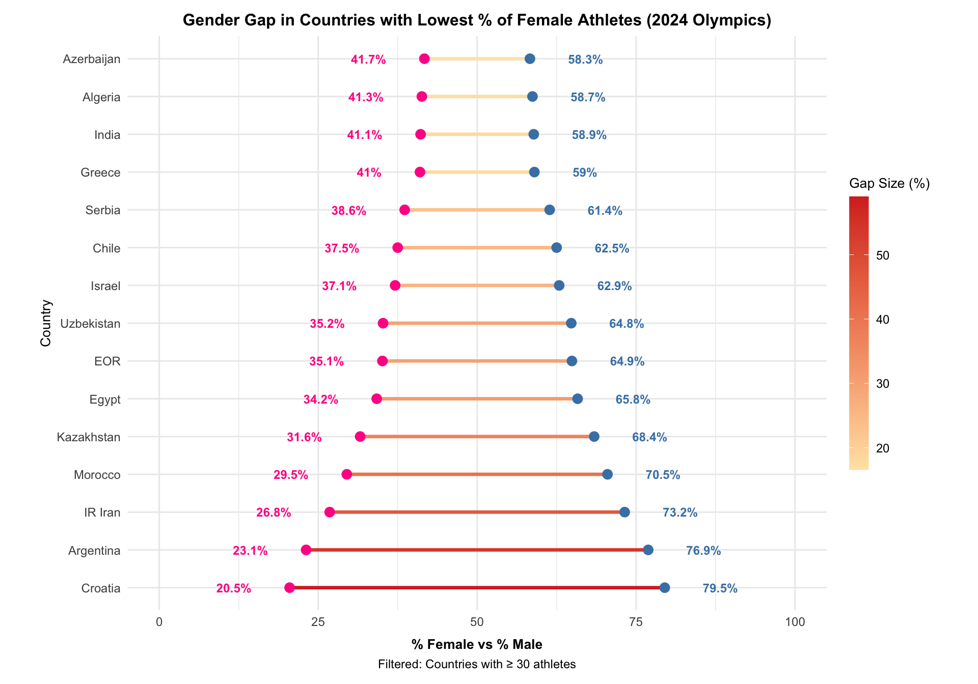
Among countries with at least 30 total athletes, which had the lowest percentage of female representation at the 2024 Olympics?

female_participation <- olympics_dfclean |>
  filter(year == 2024) |>  
  distinct(country, sex, athlete_name) |>  
  group_by(country, sex) |>
  summarise(athletes = n()) |>  
  pivot_wider(
    names_from = sex,  # Create new columns based on unique values in 'sex'
    values_from = athletes, # Fill those new columns with numbers from the athletes column
    values_fill = 0 ) |> #If country has no athletes for gender, fill with 0 instead of NA
  mutate(total = F + M,  # Create new column for total athletes per country
    percentage_female = round(F / total * 100, 1))  # % of athletes who are female

`summarise()` has grouped output by 'country'. You can override using the
`.groups` argument.

female_participation_filtered <- female_participation |>
  filter(total >= 30)

# Identify bottom 15 countries by % female athletes
bottom15 <- female_participation_filtered |>
  arrange(desc(percentage_female)) |> 
  tail(15) |>  # Sort the last 15 rows 
  arrange(percentage_female) |> 
  mutate(percentage_male = round(100 - percentage_female, 1))  # Add % male for the analysis table

# Calculate additional gender gap column
bottom15 <- bottom15 |>
  mutate(gap_size = abs(percentage_female - percentage_male))  # Add gap size column (% difference)

bottom15 

# A tibble: 15 × 7
# Groups:   country [15]
   country        F     M total percentage_female percentage_male gap_size
   <fct>      <int> <int> <int>             <dbl>           <dbl>    <dbl>
 1 Croatia       15    58    73              20.5            79.5     59  
 2 Argentina     33   110   143              23.1            76.9     53.8
 3 IR Iran       11    30    41              26.8            73.2     46.4
 4 Morocco       18    43    61              29.5            70.5     41  
 5 Kazakhstan    25    54    79              31.6            68.4     36.8
 6 Egypt         53   102   155              34.2            65.8     31.6
 7 EOR           13    24    37              35.1            64.9     29.8
 8 Uzbekistan    31    57    88              35.2            64.8     29.6
 9 Israel        33    56    89              37.1            62.9     25.8
10 Chile         18    30    48              37.5            62.5     25  
11 Serbia        44    70   114              38.6            61.4     22.8
12 Greece        41    59   100              41              59       18  
13 India         46    66   112              41.1            58.9     17.8
14 Algeria       19    27    46              41.3            58.7     17.4
15 Azerbaijan    20    28    48              41.7            58.3     16.6

Key Insight:

This analysis identifies the 15 countries with the lowest percentage of female athletes at the 2024 Summer Olympics, based on delegations with at least 30 total participants. Croatia had the lowest proportion, with women making up only 20.5% of its Olympic team. Other countries with low female representation included Argentina (23.1%), Iran (26.8%), and Morocco (29.5%).Most of these countries had less than 40% female participation, revealing that gender gaps still persist in Olympic representation in certain regions.

Question4-Visualization ️

gap_graph <- ggplot(bottom15, aes(y = reorder(country, percentage_female))) +
  # Gradient segment
  geom_segment(aes(x = percentage_female, xend = percentage_male,
                   yend = country, color = gap_size), size = 2.5) +
  
  # Gradient legend
  scale_color_gradient(low = "#FFE5B4", high = "#D73027", name = "Gap Size (%)") +
  guides(color = guide_colorbar(barheight = unit(0.4, "npc"),   
                                barwidth = unit(0.02, "npc"))) +

  # Female point
  geom_point(aes(x = percentage_female), color = "deeppink", size = 7) +
  geom_text(aes(x = percentage_female, label = paste0(percentage_female, "%")),
            color = "deeppink", size = 8, fontface = "bold",
            hjust = 1, nudge_x = -6) +

  # Male point
  geom_point(aes(x = percentage_male), color = "steelblue", size = 7) +
  geom_text(aes(x = percentage_male, label = paste0(percentage_male, "%")),
            color = "steelblue", size = 8, fontface = "bold",
            hjust = 0, nudge_x = 6) +

  # X-axis scale
  scale_x_continuous(
    limits = c(0, 100),
    expand = expansion(mult = c(0.05, 0.05))) +

  # Labels
  labs(
    title = "Gender Gap in Countries with Lowest % of Female Athletes (2024 Olympics)",
    subtitle = "Gradient lines reflect how large the gap is between male and female athletes",
    x = "% Female vs % Male",
    y = "Country",
    caption = "Filtered: Countries with ≥ 30 athletes") +


  theme_light(base_size = 25) +
  theme(
    plot.title = element_text(face = "bold", hjust = 0.5, size = 30),
    plot.subtitle = element_text(size = 25, hjust = 0.5, color = "gray40"),
    plot.caption = element_text(size = 23, hjust = 0.5), 
    legend.title = element_text(size = 18),               
    legend.text = element_text(size = 16),               
    axis.title.x = element_text(size = 20, face = "bold", margin = margin(t = 12)),  
    axis.title.y = element_text(size = 24),
    axis.text.x = element_text(size = 22),
    axis.text.y = element_text(size = 22, lineheight = 1.5),
    plot.margin = margin(15, 20, 15, 20))

Warning: Using `size` aesthetic for lines was deprecated in ggplot2 3.4.0.
ℹ Please use `linewidth` instead.

# Save the graph
ggsave("out/plot4.png", gap_graph, width = 16, height = 12, dpi = 400, units = "in")

Question5-Analysis

Among all female athletes, which ones have won the most gold medals for their country? (One top athlete per country)

#Filter only female athletes who won gold medals
top_female_gold <- olympics_dfclean |>
  filter(sex == "F", medal == "Gold") |>  

#Remove duplicates — only count unique medals by athlete, year, and event
  distinct(athlete_name, year, event, country, medal) |>

#Count the number of gold medals per athlete within each country
  group_by(country, athlete_name) |>
  summarise(gold_medals = n()) |>

#For each country, keep only the athlete with the highest gold medal count
  group_by(country) |>
  filter(gold_medals == max(gold_medals)) |>  
  filter(row_number() == 1) |>               

#Sort by number of gold medals and keep only the top 10 countries
  arrange(desc(gold_medals)) |>
  head(10)  

`summarise()` has grouped output by 'country'. You can override using the
`.groups` argument.

top_female_gold

# A tibble: 10 × 3
# Groups:   country [10]
   country        athlete_name           gold_medals
   <fct>          <chr>                        <int>
 1 Soviet Union   Larysa (diriy-)                  9
 2 New Zealand    Lisa Carrington                  8
 3 United States  Jennifer (-cumpelik)             8
 4 Czechoslovakia Vra (-odloilov)                  7
 5 Russia         Svetlana Romashina               7
 6 East Germany   Kristin Otto                     6
 7 Italy          Maria Vezzali                    6
 8 Australia      McKEON Emma                      5
 9 China          Chen Ruolin                      5
10 Germany        Birgit Fischer-schmidt           5

Key Insight:

The above analysis highlights the top-performing female Olympic athletes based on the number of gold medals won, while selecting only one top athlete per country. The athlete with the most gold medals is Larysa from the Soviet Union, with 9 golds, followed closely by Lisa Carrington (New Zealand) and Jennifer (USA), each with 8 gold medals.

Question5-Visualization ️

p3 <- ggplot(top_female_gold, aes(x = reorder(athlete_name, gold_medals), y = gold_medals, color = country)) +
  geom_segment(aes(xend = athlete_name, y = 0, yend = gold_medals), size = 1.2) +
  geom_point(size = 5) +
  coord_flip() +
  labs(title = "Top 10 Female Athletes with Most Gold Medals (One per Country)",
    subtitle = "Each line represents a country's top female gold medalist",
    x = NULL,  # Remove "Athlete" label so as to reduce overlap
    y = "Gold Medals",
    color = "Country", caption = "Source: Kaggle | Author: Brandon") +
  theme_minimal(base_size = 12) +
  theme(
    plot.title = element_text(face = "bold", hjust = 0.5),
    plot.subtitle = element_text(hjust = 0.5),
    legend.position = "right",
    axis.text.y = element_text(margin = margin(r = 10)))  # add the spacing so names will not overlap the label

p3_plotly <- ggplotly(p3)

p3_plotly

# Save the plot as a file

htmlwidgets::saveWidget(p3_plotly, "out/interactive_plot5.html", selfcontained = TRUE)

Question6-Analysis

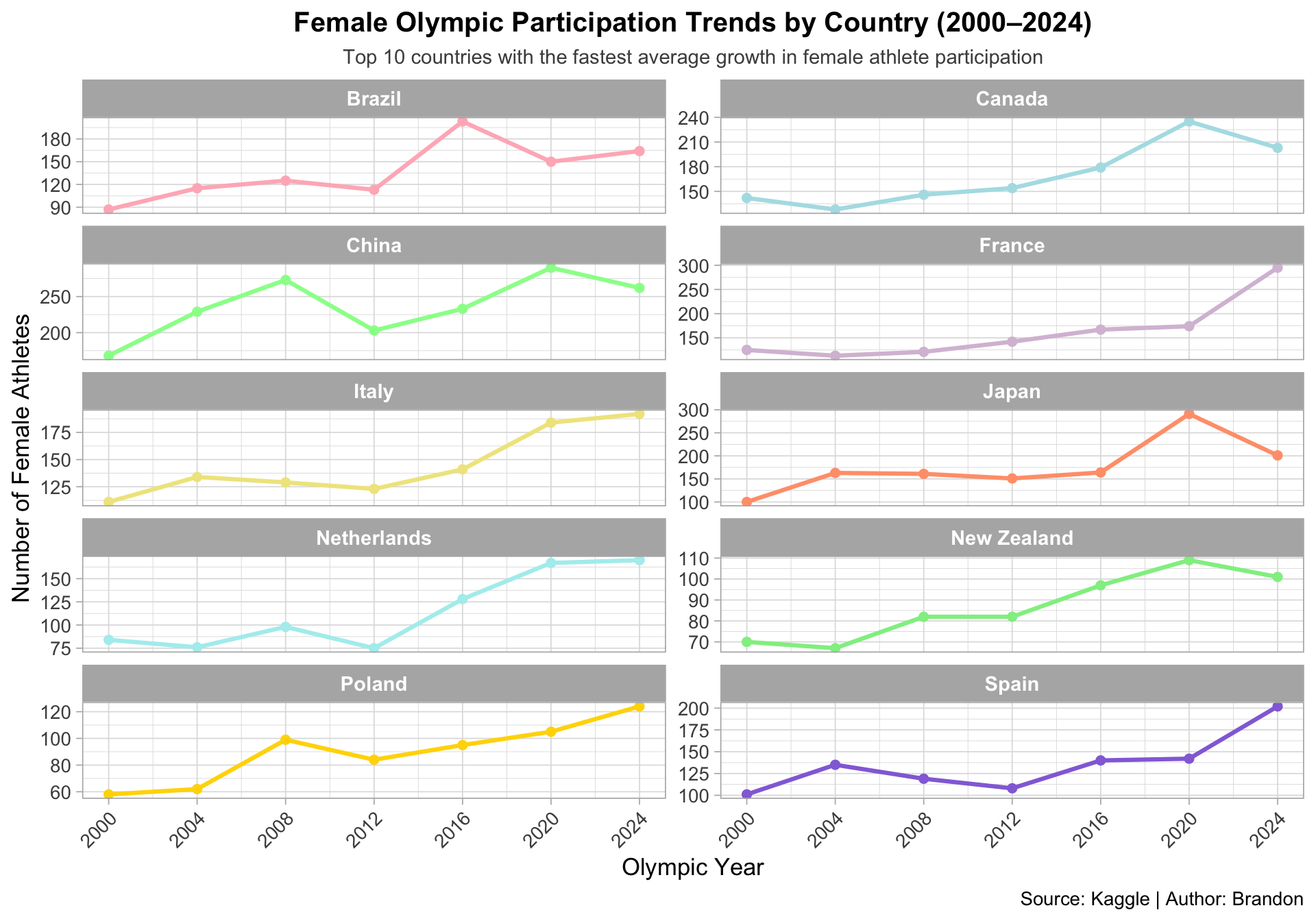
Which countries with substantial initial participation (≥ 50 female athletes in 2000s) have demonstrated the fastest average percentage growth in supporting female Olympians from 2000 to 2024?

female_growth <- olympics_dfclean |>
  filter(sex == "F", year >= 2000) |> # Scope the the focus on only the female athletes from 2000 onwards
  distinct(athlete_name, country, year) |>
  group_by(country, year) |>
  summarise(female_athletes = n()) |>
  arrange(country, year) |>
  group_by(country) |>
  summarise(
    start = first(female_athletes), # First data point (starting value like 2000)
    end = last(female_athletes),   # Last data point (ending value like 2024)
    years = n(),                  # Number of Olympic Games that take into account
    total_growth_percentage = round(((end - start) / start) * 100, 1),  # Overall % growth from first to last year 
    avg_growth_percentage = round(total_growth_percentage / (years - 1), 1),) |> # Average % growth per Olympic cycle
  filter(start >= 50, years >= 3) |> # Keep only countries that had at least 50 female athletes in the base year and appeared in at least 3 Games
  arrange(desc(avg_growth_percentage))

`summarise()` has grouped output by 'country'. You can override using the
`.groups` argument.

# Store top 10 countries into the top10 data frame 
top10_countries_df <- head(female_growth, 10)
top10_countries <- top10_countries_df$country

# Prepare trend data separately for the data visualization below
trend_data <- olympics_dfclean |>
  filter(sex == "F", year >= 2000, year <= 2024, country %in% top10_countries) |>
  distinct(athlete_name, country, year) |>
  group_by(country, year) |>
  summarise(female_athletes = n())

`summarise()` has grouped output by 'country'. You can override using the
`.groups` argument.

trend_data

# A tibble: 70 × 3
# Groups:   country [10]
   country  year female_athletes
   <fct>   <int>           <int>
 1 Brazil   2000              87
 2 Brazil   2004             115
 3 Brazil   2008             125
 4 Brazil   2012             113
 5 Brazil   2016             203
 6 Brazil   2020             150
 7 Brazil   2024             164
 8 Canada   2000             142
 9 Canada   2004             128
10 Canada   2008             146
# ℹ 60 more rows

Key Insight:

This analysis examines which countries with substantial female participation in the early 2000s (≥ 50 athletes) have achieved the fastest average growth rates in supporting female Olympians by 2024. France leads the list, growing from 125 to 295 female athletes, an average increase of 22.7% per Olympics. Poland, Netherlands, Japan, and Spain also show strong, consistent growth, each with over 16% average growth across seven Olympic Games. Some large delegations such as the United States, Germany, and Great Britain experienced more modest growth, likely due to already high participation levels in 2000.

Question6-Visualization ️

# Custom colors
line_colors <- c(
  "#FFB6C1", "#B0E0E6", "#98FB98", "#D8BFD8", "#F0E68C",
  "#FFA07A", "#AFEEEE", "#90EE90", "#FFD700", "#9370DB")

# Updated plot
p4 <- ggplot(trend_data, aes(x = year, y = female_athletes, color = country, group = country)) +
  geom_line(size = 1.2) +
  geom_point(size = 2.5) +
  scale_color_manual(values = line_colors) +
  facet_wrap(~ country, ncol = 2, scales = "free_y") +
  scale_y_continuous(labels = scales::comma) +
  scale_x_continuous(breaks = seq(2000, 2024, by = 4), expand = expansion(mult = c(0.05, 0.1))) +
  labs(
    title = "Female Olympic Participation Trends by Country (2000–2024)",
    subtitle = "Top 10 countries with the fastest average growth in female athlete participation",
    x = "Olympic Year",
    y = "Number of Female Athletes",
    caption = "Source: Kaggle | Author: Brandon") +
  theme_light(base_size = 23) +  
  theme(
    plot.title = element_text(size = 25, face = "bold", hjust = 0.5),
    plot.subtitle = element_text(size = 20, hjust = 0.5, color = "gray30"),
    axis.title = element_text(size = 20),
    axis.text.x = element_text(size = 18, angle = 45, hjust = 1),
    axis.text.y = element_text(size = 18, margin = margin(r = 15)),
    strip.text = element_text(face = "bold", size = 18),  
    legend.position = "none",
    plot.caption = element_text(size = 15))

# Save the plot 
ggsave("out/plot6.png", p4, width = 14, height = 13, dpi = 400)